Robust Production - Inventory

Consider the problem of minimizing the costs associated with inventory management while ensuring that customer demand is met consistently over a planning horizon. This approach addresses the inherant uncertainty in product demands, making it a robust optimization problem.

Taking the example introduced in Ben-Tal et al. (2004) [1], let us consider a single product inventory system which is comprised of a single warehouse and \(I\) identical factories. The planning horizon is \(T\) periods. At time period \(t\), let:

• \(d_t\) denote the demand of the product at each that is uncertain.

• \(v_t\) denote the amount of product in the warehouse at the beginning of the time period.

• \(p_t\in {\bf R}^I\) denote the amount of product to be produced during period \(t\) by each factory.

• \(c_t \in {\bf R}^I\) denote the cost of producing a unit of product at each factory at time period \(t\).

• \(p^{\rm max}\) denote the maximal production capacity for each factory at time period \(t\).

• \(q^{\rm max}\) denote the maximal cumulative production capacity for each factory.

• \(v^{\rm min}\) and \(v^{\rm max}\) denote the minimal and maximal storage capacity of the warehouse, respectively.

With this information, we can write the inventory problem as a robust linear program

\[\begin{split}\begin{array}{ll} \text{minimize} & \sum_{t=1}^{T} c_t^Tp_t \\ \text{subject to} & 0 \leq p_t \leq p^{\rm max}{\bf 1} \quad t=1,\dots,T \\ & \sum_{k = 1}^{t} p_k \leq q^{\rm max}{\bf 1} \quad t=1,\dots,T \\ & v^{\rm min} \leq v_1 + {\bf 1}^T(\sum_{k = 1}^{t} p_k) - \sum_{k = 1}^{t} d_k \leq v^{\rm max} \quad \forall (d_1,\dots, d_T) \in \mathcal{U},\quad t=1,\dots, T\\ \end{array}\end{split}\]

import numpy as np
import cvxpy as cp
import lropt
import matplotlib.pyplot as plt

Next, we consider \(I\) = 3 factories producing a product in one warehouse. The time horizon \(T\) is 24 time periods. The maximal production capacity of each one of the factories at each two-weeks period is \(P(t) = 567\), and the integral production capacity of each one of the factories for a year is \(Q = 13600\). The inventory at the warehouse should not be less then \(300\) units, and cannot exceed \(10000\) units. Initially, the inventory sits at \(500\) units.

np.random.seed(1)
T = 24 #number of periods
I = 3 #number of factories
v_min = 300
v_max = 10000
q_max = 13600
p_max = 567
v_init = 500
alphas = np.array([1, 1.5, 2])

The production cost for at period \(t\) for each factory \(i\) is given by:

\[\begin{align*} (c_t)_i = \alpha_i \left(1 - \frac{1}{2} \sin \left(\frac{\pi (t-1)}{12}\right)\right), \quad t =1,\dots,T,\quad i=1,\dots,I, \end{align*}\]

where \(\alpha = (1, 1.5, 2)\). The demand is uncertain and seasonal, reaching its peak in winter, with the following pattern,

\[\begin{split}\begin{align*} d^*_t = 1000\left(1 - \frac{1}{2} \sin \left(\frac{\pi (t-1)}{12}\right)\right), \quad t=1, 2,\dots ,T \\ \end{align*}\end{split}\]

To handle this uncertainty, we adopt the Polyhedral uncertainty set. This uncertainty set is defined by:

\[\mathcal{U}_{\text{poly}} = \{(d_1,\dots,d_T) \mid (1 - \rho) d_t^* \le d_t \le (1 + \rho) d_t^* ,\quad t=1,\dots,T\}\]

The following code defines these parameters for the problem.

def setup_parameters(proportion):
    # Check if you can use t_values here as well instead of the list comprehension
    t_values = np.arange(1, T + 1)

    c = [(alphas * (1 + 0.5 * np.sin(np.pi * (t - 1) / (T * 0.5)))).flatten() for t in range(1, T + 1)]
    c = np.array(c).T

    d_star = 1000 * (1 + 0.5 * np.sin(np.pi * (t_values - 1) / (T * 0.5)))

    lhs = np.concatenate((np.eye(T), -np.eye(T)), axis=0)
    rhs_upper = (1 + proportion) * d_star
    rhs_lower = (-1 + proportion) * d_star
    rhs = np.hstack((rhs_upper, rhs_lower))

    d = lropt.UncertainParameter(T, uncertainty_set=lropt.Polyhedral(lhs=lhs, rhs=rhs))

    return c, d, rhs_upper, rhs_lower, d_star

Next, we create a function to define the constraints of the function.

This is a function that solves the problem and returns the optimal value.

def solve_problem(d):
    p = cp.Variable((I, T), nonneg=True)
    constraints = [
        p <= p_max,
        0 <= p,
        cp.sum(p, axis=1) <= q_max
    ]

    for i in range(1, T + 1):
        constraints.append(v_min <= cp.sum(cp.sum(cp.sum(p, axis=0)[:i])) - cp.sum(d[:i]) + v_init)
        constraints.append(cp.sum(cp.sum(cp.sum(p, axis=0)[:i])) - cp.sum(d[:i]) + v_init <= v_max)

    objective = cp.Minimize(cp.sum(cp.multiply(c, p)))
    prob = lropt.RobustProblem(objective, constraints)
    prob.solve()
    return prob.objective.value, p.value

The following code calculates the robust optimal level of inventory over time.

def calculate_inventory_levels(p, rhs_upper, d_star, rhs_lower):
    low_values = []
    mid_values = []
    high_values = []
    random_trajectory = []
    for i in range(1, T + 1):
        low = (cp.sum(cp.sum(p, 0)[:i]) - cp.sum(rhs_upper[:i]) + v_init).value
        mid = (cp.sum(cp.sum(p, 0)[:i]) - cp.sum(d_star[:i]) + v_init).value
        high = (cp.sum(cp.sum(p, 0)[:i]) - cp.sum(-rhs_lower[:i]) + v_init).value

        # TODO: create random trajectory

        low_values.append(low)
        mid_values.append(mid)
        high_values.append(high)
        random_trajectory.append(np.random.uniform(low, high))
    return low_values, mid_values, high_values, random_trajectory

Finally, we define a function to plot the inventory level over time for a given value of proportion.

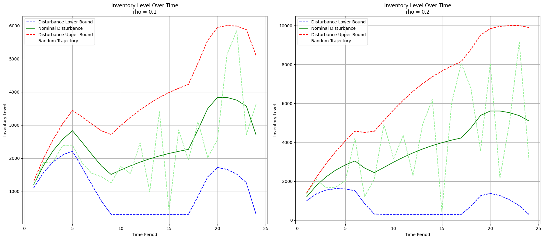
def plot_inventory_levels(ax, low_values, mid_values, high_values, random_trajectory, rho):
    ax.plot(range(1, T + 1), low_values, label='Disturbance Lower Bound', color='blue', linestyle='--')
    ax.plot(range(1, T + 1), mid_values, label='Nominal Disturbance', color='green', linestyle='-')
    ax.plot(range(1, T + 1), high_values, label='Disturbance Upper Bound', color='red', linestyle='--')
    ax.plot(range(1, T + 1), random_trajectory, label='Random Trajectory', color='lightgreen', linestyle='--')
    ax.set_xlabel('Time Period')
    ax.set_ylabel('Inventory Level')
    ax.set_title(f'Inventory Level Over Time\nrho = {rho}')
    ax.legend()
    ax.grid(True)

fig, axs = plt.subplots(1, 2, figsize=(18, 8))
rho_values = [0.1, 0.2]

for i, rho in enumerate(rho_values):
    c, d, rhs_upper, rhs_lower, d_star = setup_parameters(rho)
    optimal_value, p_value = solve_problem(d)

    print(f"rho = {rho}: The robust optimal value is {optimal_value:.3E}")

    low_values, mid_values, high_values, random_traj = calculate_inventory_levels(p_value, rhs_upper, d_star, rhs_lower)
    plot_inventory_levels(axs[i], low_values, mid_values, high_values,random_traj, rho)

plt.tight_layout()
plt.show()

/Users/mj5676/Desktop/miniconda3/envs/lropt_v3/lib/python3.12/site-packages/cvxpy/utilities/torch_utils.py:61: UserWarning: torch.sparse.SparseTensor(indices, values, shape, *, device=) is deprecated.  Please use torch.sparse_coo_tensor(indices, values, shape, dtype=, device=). (Triggered internally at /Users/runner/work/pytorch/pytorch/pytorch/torch/csrc/utils/tensor_new.cpp:643.)
  return torch.sparse.FloatTensor(i, v, torch.Size(value_coo.shape)).to(dtype)

rho = 0.1: The robust optimal value is 3.830E+04
rho = 0.2: The robust optimal value is 4.367E+04

References

1. Ben-Tal, Aharon, Alexander Goryashko, Elana Guslitzer, and Arkadi Nemirovski. 2004. Adjustable robust solutions of uncertain linear programs. Mathematical Programming 99(2) 351-376. - add a clickable link