Robust Mean - Variance Portfolio

Consider the problem of allocating to allocate a capital over multiple assets to maximize portfolio’s expected return, while ensuring a very low probability that the actual return falls below the computed value. This approach addresses the inherent uncertainty in portfolio returns, making it a robust optimization problem.

In the example taken from [1, Section 3.4], we have \(n = 200\) assets. Let \(r_i\) denote the return, and \(\sigma_i\) denote the standard deviation associated with the \(i\)-th asset. The last asset represents cash, so we set its return to \(r_{n}=1.05\) and standard deviation to \(\sigma_n = 0\). The returns of the remaining assets \(r_i\), for \(i=1,\dots, n-1\), are random variables taking values in the intervals \([\mu_i - \sigma_i ,\mu_i + \sigma_i ]\). The vectors \(\mu\) and \(\sigma\) are defined as

\[\mu_i = 1.05 + \frac{0.3\left(n - i\right)}{n - 1} , \quad \sigma_i = 0.05 + \frac{0.6\left(n - i\right)}{n - 1}, \quad i=1,\dots,n-1.\]

To solve this problem, we first import the required packages and generate the data.

import lropt
import cvxpy as cp
import numpy as np
import matplotlib.pyplot as plt
import pandas as pd

n = 200
cash_return = 1.05

#Define mu
mu = np.zeros(n)
mu[-1] = cash_return
for i in range(n - 1):
    mu[i] = cash_return + 0.3 * (n - i) / (n- 1)

#Define sigma
sigma = np.zeros(n)
for i in range(n - 1):
    sigma[i] = 0.05 + 0.6 * (n - i) / (n - 1)

The problem we want to solve is the uncertain linear optimization problem of the form

\[\begin{split}\begin{array}{ll} \text{maximize} & t \\ \text{subject to} & r^Tx \geq t \quad \forall r \in \mathcal{U} \\ & 1^T x= 1 \\ & x \geq 0, \end{array}\end{split}\]

where \(x_i\) is the normalized capital to be invested in asset \(i\), and \(r\) is the uncertain vector of returns. We model the uncertain returns as \(r_i = \mu_i + \sigma_i z_i\) for \(i=1,\dots,n\), where \(z = (z_1,\dots,z_n)\) is a vector of uncertain parameters. In the following snippet, we solve this problem using Ellipsoidal and Budget uncertainty sets of the form:

\[\begin{split}\begin{array}{ll} &\mathcal{U}_{\rm ellip} = \{ r = \mu + {\bf diag}(\sigma) z \mid \|z\|_2 \le \rho \}\\ &\mathcal{U}_{\rm budg} = \{ r = \mu + {\bf diag}(\sigma) z \mid \|z\|_{\infty} \le \rho,\; \|z\|_{1} \le \rho \},\\ \end{array}\end{split}\]

for different values of the set radius \(\rho\).

names = ['Ellipsoidal', 'Budget']
rho_values = np.linspace(0.1, 2.0, 10)  # Range of rho values

uncertainty_sets = {
    'ellipsoidal': lambda rho: lropt.Ellipsoidal(rho=rho, b=mu, a=np.diag(sigma)),
    'budget': lambda rho: lropt.Budget(rho1=rho, rho2=rho, b=mu, a=np.diag(sigma))
}

results = {}
for uc_name, uc in uncertainty_sets.items():

    results_uc = []
    for rho in rho_values:
        t = cp.Variable()
        x = cp.Variable(n)
        r = lropt.UncertainParameter(n, uncertainty_set=uc(rho))

        constraints = [
            r @ x >= t,
            cp.sum(x) == 1,
            x >= 0
        ]

        objective = cp.Maximize(t)
        prob = lropt.RobustProblem(objective, constraints)
        prob.solve()

        optimal_allocation = x.value
        optimal_return = t.value

        # Estimates of covariance and risk based on simplified model
        cov_matrix = np.diag(sigma ** 2)
        variance = np.dot(optimal_allocation.T, np.dot(cov_matrix, optimal_allocation))
        risk = np.sqrt(variance)

        results_uc.append({
            'rho': rho,
            'return': optimal_return,
            'risk': risk
        })

    results[uc_name] = pd.DataFrame(results_uc)

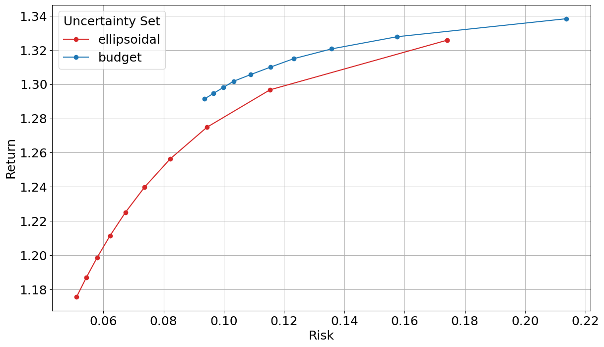
The following code creates a graph of the tradeoff curve of risk and return over a range of values of \(\rho\).

plt.figure(figsize=(14, 8))
plt.rcParams.update({"font.size": 18})
colors = ['tab:red', 'tab:blue']

for idx, uc in enumerate(uncertainty_sets.keys()):
    plt.plot(results[uc]['risk'], results[uc]['return'], color=colors[idx], marker='o', label=uc)

plt.xlabel('Risk')
plt.ylabel('Return')
plt.legend(title='Uncertainty Set')
plt.grid(True)
plt.show()

References

1. Bertsimas, Dimitris, and Dick Den Hertog. Robust and Adaptive Optimization. [Dynamic Ideas LLC], 2022.